반응형
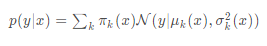
MDN에서는 출력값을 명시적으로 생성하여 x->y 매핑을 모델링하는 대신
각 대상의 확률 분포를 학습하고 출력을 샘플링한다.
분포 자체는 여러 가우시안(가우스 혼합) 으로 표시된다.
모든 입력 x에 대해 distribution parameters를 학습한다. mean, variance, mixing coefficient
k : 가우시안 수
l : 입력 피처 수 (l + 2) k
출력값:
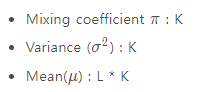
the mixing coefficients와 component density parameters를 학습한다.
# In our toy example, we have single input feature
l = 1
# Number of gaussians to represent the multimodal distribution
k = 26

# Network
input = tf.keras.Input(shape=(l,))
layer = tf.keras.layers.Dense(50, activation='tanh', name='baselayer')(input)
mu = tf.keras.layers.Dense((l * k), activation=None, name='mean_layer')(layer)
# variance (should be greater than 0 so we exponentiate it)
var_layer = tf.keras.layers.Dense(k, activation=None, name='dense_var_layer')(layer)
var = tf.keras.layers.Lambda(lambda x: tf.math.exp(x), output_shape=(k,), name='variance_layer')(var_layer)
# mixing coefficient should sum to 1.0
pi = tf.keras.layers.Dense(k, activation='softmax', name='pi_layer')(layer)
model = tf.keras.models.Model(input, [pi, mu, var])
optimizer = tf.keras.optimizers.Adam()
model.summary()
Loss
https://www.katnoria.com/mdn/
Mixture Density Networks Supervised machine learning models learn the mapping between the input features (x) and the target values (y). The regression models predict continuous output such as house price or stock price whereas classification models predict
www.katnoria.com
반응형
'Machine Learning > 딥러닝' 카테고리의 다른 글
| [Keras] Noise Regularization (0) | 2019.08.27 |
|---|---|
| 훈련셋, 검증셋, 시험셋 (0) | 2019.08.26 |
| Validation, Test 데이터세트 비교 (0) | 2019.08.24 |
| 딥러닝 모델의 교차검증 (Cross Validation) (0) | 2019.08.21 |
| [Machine Learning] Train data normalization (1) | 2019.07.12 |
